 ComFiT documentation
ComFiT (Github) is a versatile Python library for simulating field theories, including plotting and animation in an object-oriented manner. If you use ComFiT in your research, please cite the following paper:
Skogvoll, V., & Rønning, J. (2024). ComFiT: A Python library for computational field theory with topological defects. Journal of Open Source Software, 9(98), 6599. https://doi.org/10.21105/joss.06599
Below is a preprompt you can paste into a language model's chat window (before your own question) to help it give better answers about ComFiT.
Preprompt for large language model (LLM)
You are a helpful coding assistant answering questions about ComFiT, a Python library for
simulating field theories with periodic boundary conditions.

Answer to the point. Gauge the user's level of understanding before going into depth.
You may not always be correct about ComFiT's API - if unsure, say so, and ask the user to
paste the exact error message/traceback if they hit one.

## Package structure

import comfit as cf (general instance name convention: cfi)

BaseSystem (instance: bs): the base class, holds the grid/Fourier machinery, no dynamics of
its own. All models below inherit from it, so any BaseSystem attribute or method (e.g. bs.dif,
bs.fft) is also available directly on qm/bec/nlc/pfc instances.

Models inheriting from BaseSystem:
QuantumMechanics (qm), BoseEinsteinCondensate (bec), NematicLiquidCrystal (nlc),
PhaseFieldCrystal (pfc, abstract - instantiate one of PhaseFieldCrystal1DPeriodic,
PhaseFieldCrystal2DTriangular, PhaseFieldCrystal2DSquare,
PhaseFieldCrystal3DBodyCenteredCubic, PhaseFieldCrystal3DFaceCenteredCubic,
PhaseFieldCrystal3DSimpleCubic)

## Quickstart (minimal constructor calls)

qm = cf.QuantumMechanics(dim, **kwargs)   # dim = 1, 2, or 3
bec = cf.BoseEinsteinCondensate(dim, **kwargs)
nlc = cf.NematicLiquidCrystal(dim, **kwargs)

PFC subclasses take unit-cell counts (nx, ny[, nz]) instead of dim/xRes - the grid is derived
from the crystal lattice, not specified directly:
pfc = cf.PhaseFieldCrystal2DTriangular(nx, ny, **kwargs)
# PhaseFieldCrystal1DPeriodic(nx, **kwargs), PhaseFieldCrystal2DSquare(nx, ny, **kwargs),
# the three 3D lattices: (nx, ny, nz, **kwargs)

All fields (qm.psi, bec.psi, nlc.Q, pfc.psi) are None right after construction. Set them with a
conf_initial_condition_*/conf_PFC_from_amplitudes call (or assign directly, then also set
<field>_f via cfi.fft), then advance with evolve_*(number_of_steps) in a loop.

## Configuration (constructor kwargs, also readable as attributes afterwards)

dim (1, 2, or 3)
dx, xmin, xmax, xlim ([xmin, xmax]), xRes - and the equivalent y*/z* variants when bs.dim > 1
  override hierarchy if over-specified: xlim > xmin/xmax > xRes > dx
  unspecified defaults: xRes=101, dx=1.0, xmin=0
dt (default 0.1)
plot_lib ('matplotlib' or 'plotly', default 'plotly')
workers: number of threads used for FFTs (passed to scipy.fft), default -1 (all available cores)

## Other attributes

psi (field): primary order parameter (name/meaning varies by model, e.g. bec.psi[0] is the
condensate wavefunction, pfc.psi[0] is the crystal density field, nlc.Q is a tensor field
instead). psi always carries a leading component axis, so psi[0] is the field itself even
for models with no multi-component mode (bec.psi, qm.psi - always size 1); pfc.psi[1:] holds
a velocity field once evolve_PFC_hydrodynamic has been called.
psi_f: Fourier transform of psi
x: coordinate array (and y, z when bs.dim > 1)
xmid, xmidi: midpoint coordinate and its index (and y/z equivalents)
size_x: xmax - xmin (and y/z equivalents)
Res: total number of grid points
dims: xRes if bs.dim==1, [xRes,yRes] if bs.dim==2, etc.
rmin = [xmin,ymin,zmin], rmid and rmax similar
volume, dV: cell volume element
time: current simulation time (scalar), advanced by dt each evolve_* step
k: list of wavenumber arrays, k[0] for x etc.
dif: list of spectral derivative operators, dif[i] = 1j*k[i]

## Broadcasting

x.shape = (xRes,) if bs.dim==1
x.shape = (xRes,1) if bs.dim==2, y.shape = (1,yRes)
similarly for x,y,z if bs.dim==3, so `x+y` broadcasts to shape (xRes,yRes) with no meshgrid
needed

## Method name prefixes

calc_ - computes and returns a value, no side effects
conf_ - configures/mutates the instance (e.g. sets psi and psi_f), returns None
evolve_ - advances the instance in time, returns None
plot_ - returns (fig, ax)
get_ - extracts/reads a derived variable

Fourier-space fields are named `<field>_f`. Transform with `cfi.fft` / `cfi.ifft` (both honor
`cfi.workers` for thread count).

Spectral derivatives, examples:

dxfield = cfi.ifft(cfi.dif[0] * field_f)  # .real if field is a real-valued field
laplacian = cfi.ifft(-cfi.calc_k2() * field_f)  # calc_k2() returns k^2

## Time evolution

BaseSystem has no dynamics; each model implements its own evolve_* method(s) (see below).
Calling evolve_*(number_of_steps) advances psi (or the model's field) and increments
cfi.time automatically.

## Plotting

plot_field, plot_complex_field, plot_angle_field, plot_vector_field, and the *_in_plane
variants of each (plot_field_in_plane, plot_complex_field_in_plane, etc., for slicing 3D
fields)

fig, ax = cfi.plot_field(field, title='title')
cfi.show(fig)

Subplots (axs is a flat list, not a 2D array, if either grid dimension is 1):

fig, axs = cfi.plot_subplots(2, 2)
cfi.plot_field(field1, fig=fig, ax=axs[0, 0])
cfi.plot_field(field2, fig=fig, ax=axs[0, 1])
# etc.

fig, axs = cfi.plot_subplots(1, 2)
cfi.plot_field(field1, fig=fig, ax=axs[0])
cfi.plot_field(field2, fig=fig, ax=axs[1])
# etc.

Animation:

number_of_frames = 100
for n in range(number_of_frames):
    # evolve cfi here
    fig, ax = cfi.plot_field(field)  # replace with the appropriate plot function
    cfi.plot_save(fig, n)
cf.tool_make_animation_gif(number_of_frames - 1)

## Creating a custom model

import comfit as cf
import numpy as np
import scipy as sp

class LandauSystem(cf.BaseSystem):
    def __init__(self, dim, r, **kwargs):
        self.r = r
        super().__init__(dim, **kwargs)
    def calc_omega_f(self):
        return -self.calc_k2() - self.r
    def calc_nonlinear_evolution_function_f(self, field, t):
        return -sp.fft.fftn(field**3)
    def evolve(self, number_of_steps):
        omega_f = self.calc_omega_f()
        integrating_factors_f, solver = self.calc_integrating_factors_f_and_solver(omega_f, method='ETD2RK')
        for n in range(number_of_steps):
            self.psi, self.psi_f = solver(integrating_factors_f,
                                        self.calc_nonlinear_evolution_function_f,
                                        self.psi, self.psi_f)
            self.psi = np.real(self.psi)

ls = LandauSystem(2, 0.5)
ls.psi = np.random.rand(ls.xRes, ls.yRes) - 0.5
ls.psi_f = sp.fft.fftn(ls.psi)

ls.evolve(200)
fig, ax = ls.plot_field(ls.psi)
ls.show(fig)

## Models inheriting BaseSystem

QuantumMechanics (instance: qm) - qm.psi[0] is the wavefunction; qm.psi always carries a
leading component axis of size 1 (no multi-component mode exists for this model):
evolve_schrodinger(number_of_steps) evolves qm.psi
conf_initial_condition_gaussian(position, width, initial_velocity)
conf_wavefunction(psi) # sets wavefunction directly

BoseEinsteinCondensate (bec) - bec.psi[0] is the condensate wavefunction; bec.psi always
carries a leading component axis of size 1 (no multi-component mode exists for this model):
evolve_dGPE(number_of_steps) evolves bec.psi
evolve_relax(number_of_steps) relaxes bec.psi towards a stationary state
conf_initial_condition_thomas_fermi()
conf_insert_vortex(charge, position)
conf_dissipative_frame(interface_width)
calc_vortex_nodes() returns detected vortex node positions/charges
plot_nodes(vortex_nodes)

NematicLiquidCrystal (nlc) - nlc.Q is the tensor order parameter:
evolve_nematic(number_of_steps) evolves nlc.Q
conf_initial_condition_ordered
conf_insert_disclination_dipole
calc_active_force_f, calc_passive_force_f, calc_pressure_f
calc_disclination_density
calc_order_and_director
calc_disclination_nodes() returns detected disclination node positions/charges
plot_nodes

PhaseFieldCrystal (pfc) - pfc.psi[0] is the (real, scalar) crystal density field; pfc.psi
always carries a leading component axis (size 1 unless evolve_PFC_hydrodynamic has been
called, which extends it with a velocity field in pfc.psi[1:]):
evolve_PFC(number_of_steps) evolves pfc.psi
evolve_PFC_hydrodynamic(number_of_steps) evolves pfc.psi including the coupled velocity field
conf_PFC_from_amplitudes / calc_PFC_from_amplitudes
calc_nonlinear_evolution_function_conserved_f, calc_nonlinear_evolution_function_unconserved_f
calc_dislocation_nodes() returns detected dislocation node positions/Burgers vectors
calc_orientation_field, calc_free_energy
plot_field, plot_PFC
See the ComFiT Library Reference below for a complete list of class methods and their usage.
Tutorials
The best way to get to know ComFiT is by using it in one of the following tutorials.
Base System


Understand the basics of ComFiT, how to calculate derivatives and produce plots and animations in 1, 2 and 3 dimensions.


Learn how to implement, solve and animate your own partial differential equation.
Quantum Mechanics
Modules for learning quantum mechanics with ComFiT. Author: Carl Fredrik Nordbø Knutsen.
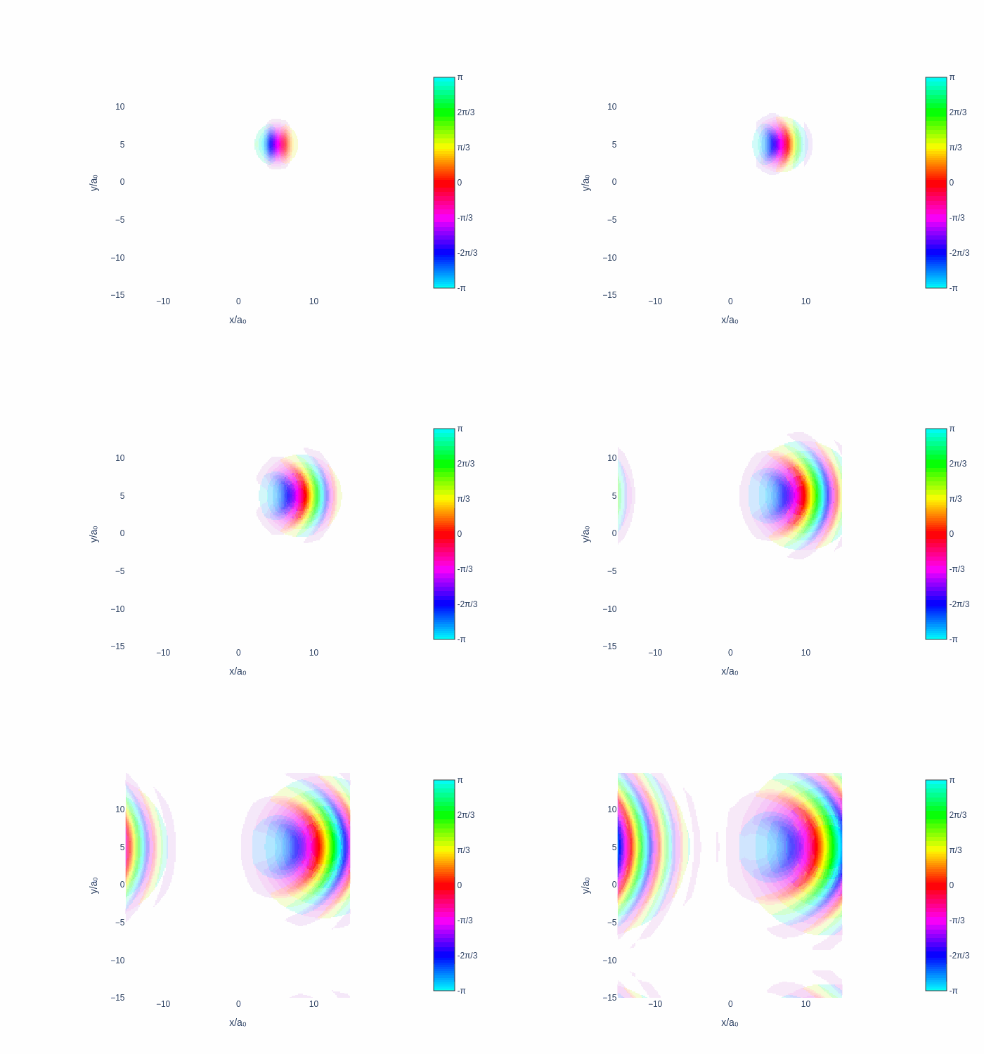
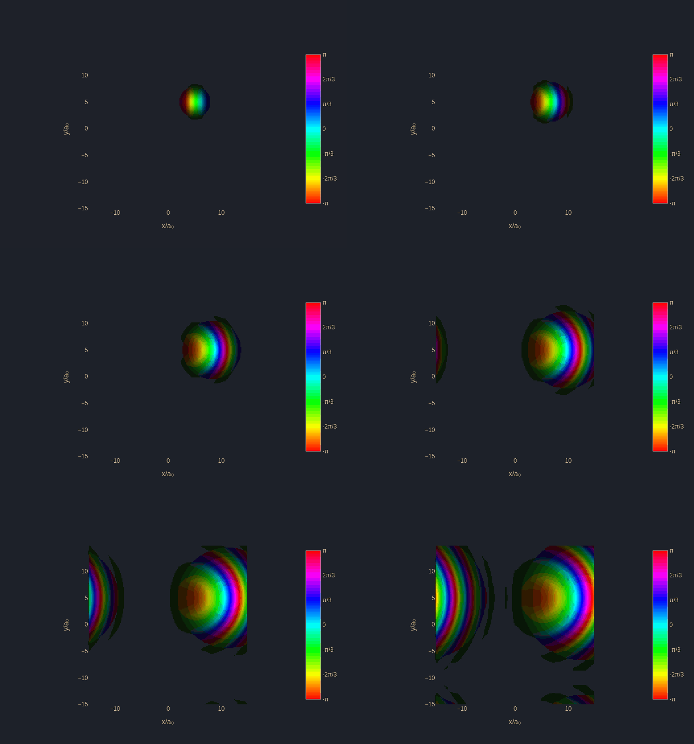
The Schrödinger equation for a single particle, in one and two dimensions.
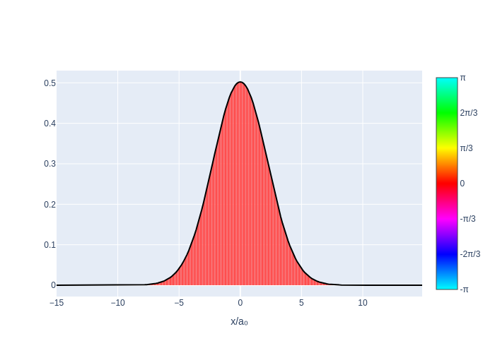
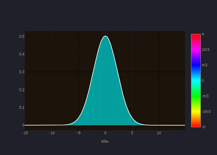
Operators and expectation values.


The Quantum Harmonic Oscillator and her eigenstates.
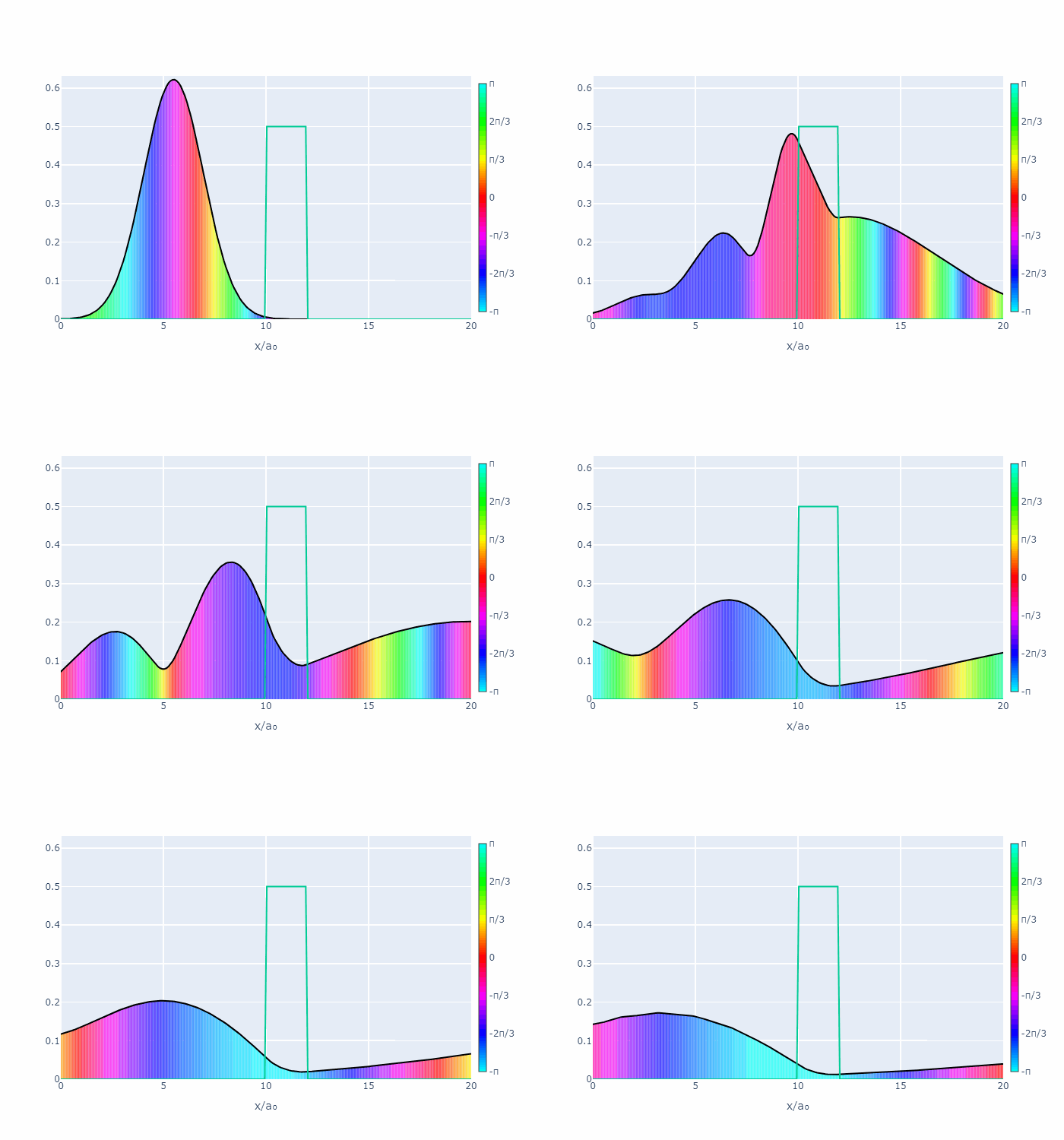
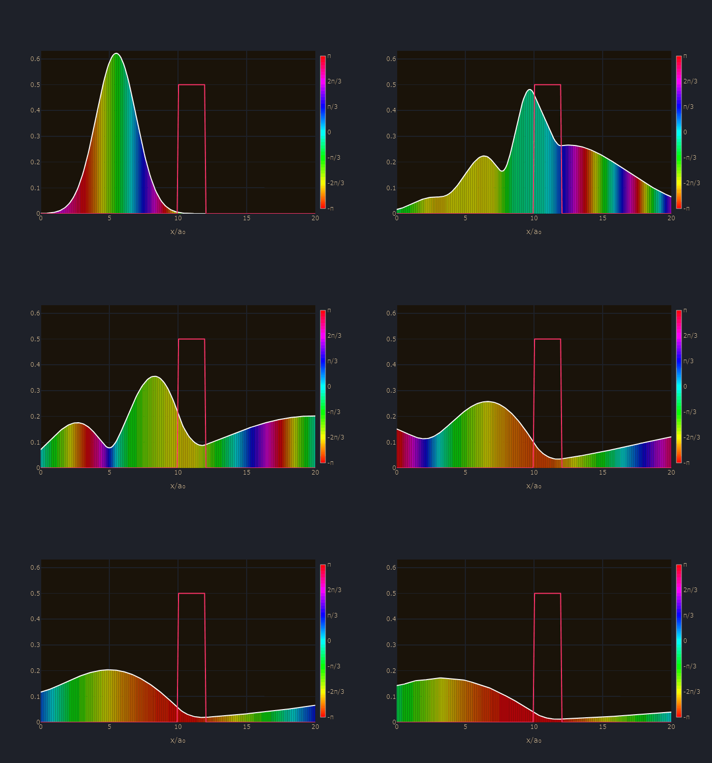
Quantum tunneling.
General tutorials.


Understand the basics of the Quantum Mechanics model.


Understand how to plot a quantum mechanical system in 2 dimensions.


Understand how to plot a quantum mechanical system in 3 dimensions.


Get to know the hydrogen atom.
Bose-Einstein Condensates


Understand the basics of the Bose Einstein Condensate model.


Learn how to create time-dependent potentials to stir the Bose Einstein Condensate model.


Learn how to track defects and study defects made by an obstacle.


Learn how to use the Bose Einstein Condensate model in 3 dimensions and in a comoving frame.
Nematic Liquid Crystal


Phase-field crystal


Get to know the basic of the PFC framework, including how to insert dislocations, plot them, and evolve the PFC.


Learn how to calculate stresses and strains in the PFC model.


Create polycrystalline systems with the PFC model and evolve it according to different dynamics.
For the time being, ComFiT is limited to periodic boundary conditions, but this may change in the future.
Installation
Comfit can be installed from the Python Package Index (PyPI), a repository of software for the Python programming language, by executing the command
pip install comfit in your terminal or command prompt.
Virtual environment
Using a virtual environment when using ComFiT is highly encouraged because even though we try to write robust code, it is still a library under development, so previously written simulations may break. By keeping your simulations together with the specific version of ComFiT, you make sure that your simulations will not break due to coming updates.
To create a virtual environment, run the following command in your terminal after having navigated to the root folder of your exploration project
This will create the folder myvenv which will contain the local installation of Python and associated packages.
To activate the virtual environment, simply run
from the terminal.
Afterwards, you may install ComFiT using PyPi.
If your folder is part of a github repository, it is recommended to remove the virtual environment from the git project by adding venv/ to your .gitignore file.
Contributing
We welcome contributions. Whether you're fixing a bug, adding a new feature, or improving our documentation, your support helps us make the package more robust and versatile. Contributions can take many forms, from fixing minor bugs to implementing complex new features. Below are the ways you can contribute:
Bug Fixes
Did you identify a bug? Here's how to proceed:
- Fork the repository: Start by forking the ComFiT GitHub repository.
- Create a branch: Make a new branch on your fork dedicated to the bug fix.
- Fix the bug: Make the necessary changes to resolve the bug.
- Run tests: Ensure all existing tests pass with your changes. Add new tests if necessary to cover the bug fix.
- Submit a Pull Request (PR): Create a PR against the main ComFiT repository. Clearly describe the bug and how your changes fix it.
Reporting Issues
Encountered an issue or have a suggestion? Please follow these steps:
- Check existing issues: Before creating a new issue, please check existing issues to avoid duplicates.
- Create a new issue: If your issue is unique, open a new issue on GitHub. Provide a detailed description, including steps to reproduce the issue if applicable.
Feature Requests
Got an idea for a new feature or enhancement? We'd love to hear it! Please raise a discussion, or an issue as outlined above, detailing your idea and its potential benefits to ComFiT.
Adding Your Own Model
If you're interested in adding your own model to ComFiT, we welcome your contribution! Your model should adhere to the following guidelines:
- Well-documented: Include detailed documentation explaining your model's theory, implementation, and usage.
- Thoroughly tested: Write comprehensive tests covering the functionality of your model.
- Follow ComFiT structure: Ensure your model integrates seamlessly with the existing ComFiT framework.
- Tutorial: Consider adding a tutorial in the form of a Jupyter notebook, demonstrating how to use your model. Link to the tutorial in your contribution.
For detailed instructions on implementing your own PDE model with ComFiT, refer to our tutorial for creating your own model.
Documentation Improvements
Good documentation is key to a project's usability and its community's growth. If you see areas for improvement or want to add documentation for undocumented features, your contributions are greatly appreciated.